The Law of Large Numbers. Foundation of Probability Theory

The Law of Large Numbers (LLN) is one of the most fundamental theorems in probability theory and statistics. It describes the result of performing the same experiment a large number of times and provides the theoretical foundation for statistical inference and practical applications ranging from insurance to casino gambling.

1765105273226-Pasted image 20251116182040.png

Intuitive Understanding

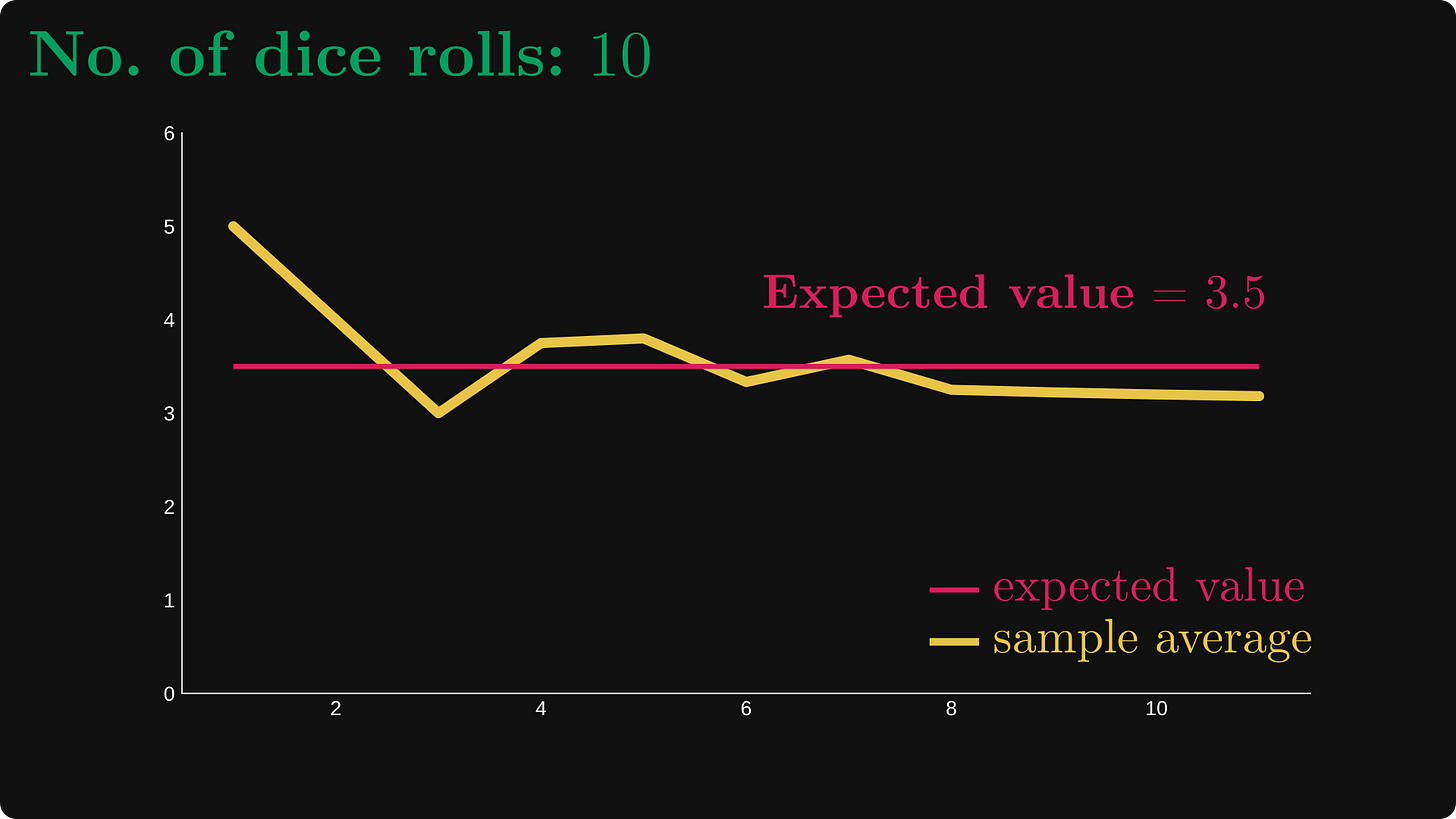
The basic idea behind the Law of Large Numbers is straightforward: as we increase the number of trials in a random experiment, the average of the results tends to get closer to the expected value. For example, if you flip a fair coin many times, the proportion of heads will approach 0.5 as the number of flips increases.

Mathematical Formulation

Let $X_1, X_2, X_3, \ldots, X_n$ be a sequence of independent and identically distributed (i.i.d.) random variables with:

Expected value: $E[X_i] = \mu$
Variance: $\text{Var}(X_i) = \sigma^2 < \infty$

The sample mean is defined as:

$\bar{X}$

Weak Law of Large Numbers (WLLN)

The Weak Law states that the sample mean converges in probability to the expected value. Formally:

$\lim_{n \to \infty} P\left(|\bar{X}_n - \mu| > \varepsilon\right) = 0$

for any $\varepsilon > 0$ .

This can also be written as:

$\bar{X}_n \xrightarrow{P} \mu \quad \text{as} \quad n \to \infty$

Proof Using Chebyshev's Inequality

We can prove the WLLN using Chebyshev's inequality. First, note that:

$E[\bar{X}_n] = \mu$

$\text{Var}(\bar{X}_n) = \frac{\sigma^2}{n}$

Applying Chebyshev's inequality:

$P\left(|\bar{X}_n - \mu| \geq \varepsilon\right) \leq \frac{\text{Var}(\bar{X}_n)}{\varepsilon^2} = \frac{\sigma^2}{n\varepsilon^2}$

As $n \to \infty$ , the right side approaches 0, proving the theorem.

Strong Law of Large Numbers (SLLN)

The Strong Law provides a stronger form of convergence—almost sure convergence:

$P\left(\lim_{n \to \infty} \bar{X}_n = \mu\right) = 1$

This means that with probability 1, the sample mean will converge to the true mean as the sample size grows to infinity.

Convergence Rate

The rate at which the sample mean converges to the expected value can be quantified. For large $n$ :

$\bar{X}_n - \mu \approx O\left(\frac{1}{\sqrt{n}}\right)$

More precisely, by the Central Limit Theorem:

$\sqrt{n}(\bar{X}_n - \mu) \xrightarrow{d} N(0, \sigma^2)$

This means that the error decreases proportionally to $\frac{1}{\sqrt{n}}$ .

Practical Example: Coin Flipping

Consider flipping a fair coin where $X_i = 1$ for heads and $X_i = 0$ for tails.

$E[X_i] = \mu = 0.5$
$\text{Var}(X_i) = \sigma^2 = 0.25$

After $n$ flips, the proportion of heads is:

$\hat{p}$

The standard error of this estimate is:

$SE = \sqrt{\frac{0.25}{n}} = \frac{0.5}{\sqrt{n}}$

For example:

After 100 flips: $SE = 0.05$
After 10,000 flips: $SE = 0.005$
After 1,000,000 flips: $SE = 0.0005$

Applications

The Law of Large Numbers has numerous practical applications:

Insurance Industry: Insurance companies rely on LLN to predict claim frequencies. While individual claims are unpredictable, the average over millions of policies converges to a predictable value.

Quality Control: Manufacturing processes use LLN to estimate defect rates. A large sample provides a reliable estimate of the true defect proportion.

Monte Carlo Methods: Numerical integration and simulation techniques use LLN to estimate expected values through random sampling:

$E[g(X)] \approx \frac{1}{n}\sum_{i=1}^{n} g(X_i)$

Gambling: Casinos profit because LLN guarantees that over many games, the house edge will manifest itself. Individual outcomes vary, but the long-run average favors the house.

Common Misconceptions

The Gambler's Fallacy: LLN does not mean that short-term deviations will be "corrected." If a coin lands heads 10 times in a row, the probability of the next flip being heads is still 0.5. The law applies to the long-run average, not to individual outcomes.

Sample Size Requirements: There is no universal "large enough" sample size. The required $n$ depends on the variance of the distribution and the desired precision.

Computational Demonstration

import random
import matplotlib.pyplot as plt

# Coin flip simulation
def simulate_coin_flips(n_flips):
    """Returns a list of cumulative averages after each flip"""
    cumulative_avg = []
    heads_count = 0
    
    for i in range(1, n_flips + 1):
        # 1 = heads, 0 = tails
        flip = random.randint(0, 1)
        heads_count += flip
        cumulative_avg.append(heads_count / i)
    
    return cumulative_avg

# Parameters
n_flips = 10000
true_probability = 0.5

# Run simulation
averages = simulate_coin_flips(n_flips)

# Visualization
plt.figure(figsize=(10, 6))
plt.plot(range(1, n_flips + 1), averages, label='Proportion of heads', alpha=0.7)
plt.xlabel('Number of flips')
plt.ylabel('Proportion of heads')
plt.title('Law of Large Numbers: Coin Flipping Simulation')
plt.legend()
plt.xscale('log')
plt.grid(True, alpha=0.3)
plt.show()

# Print statistics
print(f"After {n_flips} flips:")
print(f"Proportion of heads: {averages[-1]:.4f}")
print(f"Deviation from 0.5: {abs(averages[-1] - 0.5):.4f}")

Conclusion

The Law of Large Numbers bridges the gap between theoretical probability and empirical observation. It assures us that randomness, when observed over sufficiently many trials, exhibits predictable patterns. This theorem remains indispensable in statistics, finance, physics, and any field where understanding aggregate behavior from individual random events is essential.

The mathematical elegance of LLN lies in its generality: regardless of the underlying distribution (provided it has finite mean and variance), the same convergence behavior emerges, demonstrating a deep order within apparent randomness.